Japanese
TOP PAGE Technical Information

	[What is PERIOMATIC™] About measuring velocity, the superiority of interval method from pulse interval has been known since long ago. But its difficulty was big demerit. 　So, we COCORESEARCH succeeded to put it practical use leading in the world. The theory of PERIOMATIC ™ The pulse interval is reciprocal to frequency. To obtain output voltage proportional to input pulse frequency, we have to introduce the reciprocal computation. The figure below shows a relationship input pulse train and analogue output voltage. Here, output voltage is reciprocal to pulse interval of course.
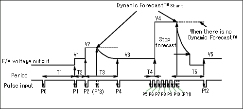
	Stage 1 : The first pulse P-0 appear initially, the period is not defined. So, the output is still zero. Stage 2 : When the next pulse P-1 comes the output V-1 calculated proportional to reciprocal value of pulse interval (period) T-1 appears. Stage 3 : By coming pulse P-2, the output V-2 appears. Here, the output V2 becomes higher than V-1 by reason of the interval T-2 is shorter than T-1. Stage 4 : If the P-3 makes same interval as T-2, the output still remain same voltage. Stage 5 : If the following pulse delayed as P-4, the hyperbola forecast computation begins from time point of imaginary pulse P-3. (The 2 reciprocal numbers are relationship of right angle hyperbola.) Stage 6 : The next pulse P-4 freezes a point of hyperbola forecasting curve. The voltage of the point is V-3, which is equal to reciprocal value of T-3. Stage 7 : If the many-fold of sudden increase of incident frequency, the analogue output rises to V-4 corresponding input change shown T-4. When the pulses continue in a same period the output keeps a voltage with no ripple shown in V-4. Stage 8 : For input pulse stop the hyperbola forecast starts after last pulse interval from last pulse. And after a settled timing the output voltage is cut down to zero as stop forecast. The settled timing is given as a coefficient of stop forecast. Actually the coefficient is given an integer. In all over applicable range, the forecast is done in relation to input frequency to obtain optimum operation. Stage 9 : If an input pulse P12 came after long period of stop reaction, an output V5 is given soon because of defined interval T5 that is determined with last pulse and new pulse P12.
	Above-mentioned forecasts are called DYNAMICFORECAST™
	* Explanation * Period = time between input pulses Frequency = 1/period

All Rights Reserved, Copyright(C) 1996-2005, COCORESEARCH INC.