Glossary [Rotation, Speed Measurement, and Pulses] >Technical Info List >Product List >HOME
What is Periomatic?
| A cycle-based frequency measurement technology originally developed by COCORESEARCH as a world first. ・Equipped with Dynamic Prediction (hyperbolic prediction) and Stop Prediction. ・Handles sudden changes from startup to stop, ultra-low to high speeds, and rapid acceleration/deceleration. ・Achieves high precision and fast response under all conditions. |
|
| For more information, please see this link > |
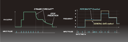
Dynamic Prediction NEW
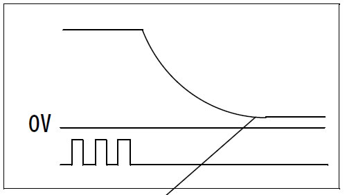
When measuring from the period of the input signal, if the input frequency (speed) drops, the system cannot respond until the next pulse arrives.
Dynamic Prediction judges a speed drop as soon as the next pulse input is even slightly later than the previous cycle, and starts hyperbolic prediction calculation.
This curve matches the value that should be confirmed at the next pulse.
| Frequency | 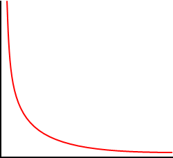 |
| Time |
[Example of Dynamic Prediction Operation Image]
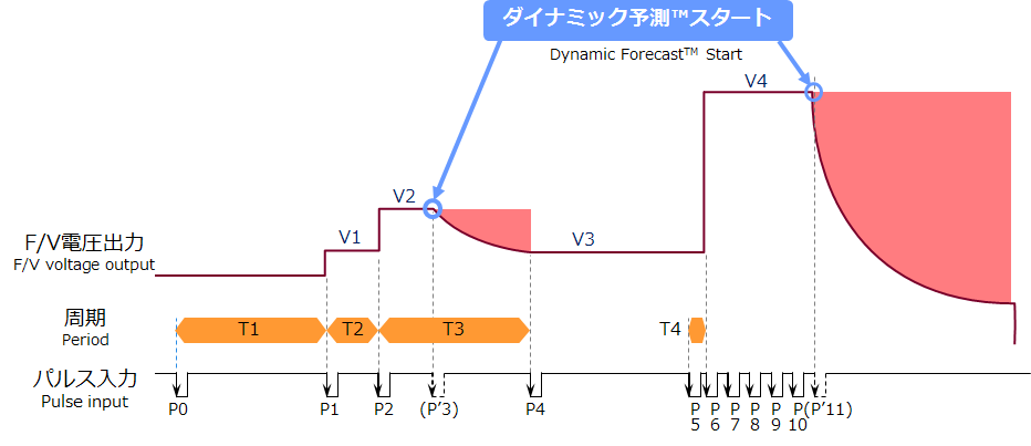
While the next pulse does not arrive, hyperbolic prediction continues indefinitely, as shown in Fig. 2 "Continuous Prediction."
It provides accurate output during long pulse periods at ultra-low speeds, and responds quickly to output zero during sudden stops from high speeds.
Since it predicts based on changes in the input pulse cycle just before stopping, there is no risk of losing dynamic range.
F/V converters capable of measuring down to low frequencies cannot distinguish between low frequency and input stop.
Therefore, to respond quickly to both low frequencies and sudden stops from high speed, Dynamic Prediction can be set to "None (Cycle Hold)," "Continuous Prediction," or "Stop Prediction" depending on the situation.
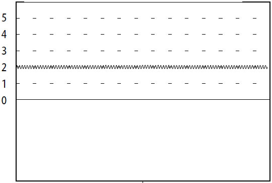
| [None (Cycle Hold Measurement)] Holds measurement data for each cycle. Does not perform prediction calculation or stop response. |
 |
| [Fig. 1] Cycle Hold Measurement | |
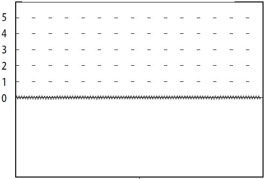
| [Continuous Prediction] Performs only prediction calculation when the frequency drops. Therefore, when no pulse is input, the curve prediction continues according to the width of the dynamic range as shown in Fig. 2, and stop prediction is not performed. |
 |
| [Fig. 2] Continuous Prediction | Indefinite Asymptote |
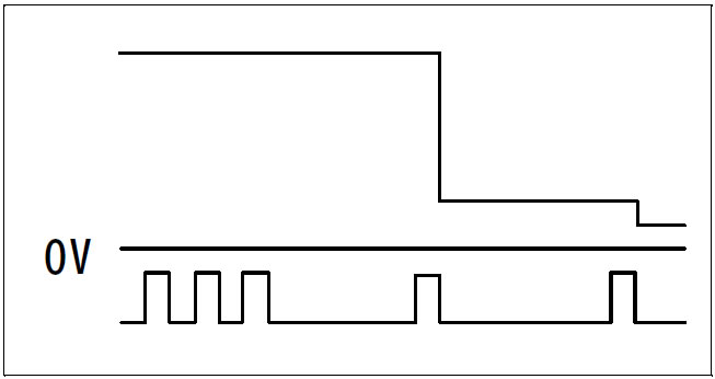
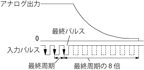
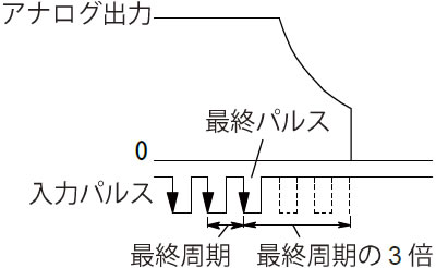
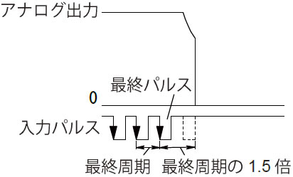
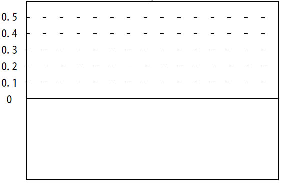
[Stop Prediction] Performs stop prediction and sudden stop detection. The larger the setting value, the faster the responsiveness to input stop.
If a stop occurs but is not detected, increase the value; if it is detected before stopping, decrease the value.
If movement resumes after a stop response, correct output is immediately obtained through the measurement calculations that were proceeding internally.
| Stop Prediction (Low Speed) | Stop Prediction (Medium Speed) | Stop Prediction (High Speed) | ||
 |
 |
 |
Ratematic (Input Frequency Rate and Display Rate Settings)
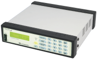
With the TDP-49/39 series, etc., you can convert and display desired physical quantities simply by setting the input frequency rate and the corresponding display rate.
To use it simply as a frequency meter in Hz, set the input frequency rate to "1" and the display rate to "1" to display the input frequency as is.
Basic Concept
Set the [Input Frequency Rate] for the number of pulses per second (Hz) and the [Display Rate] for the value you want to display.
[Setting Examples]
Ex 1) Using as a frequency meter (1 pulse input per second)
Input Frequency Rate = 1
Display Rate = 1
Ex 2) Using a 100 P/R rotary encoder to display in rpm
Input Frequency Rate = 100 [100Hz for 1 rotation per second]
Display Rate = 60 [1 rotation/s = 60 rotation/min]
Ex 3) Using a 0.12538 mL/P flow sensor to display in L/min
For an input of 1Hz (1 pulse per second), find the flow rate per minute (mL/min). 0.12538 mL/s × 60s = 7.5228 mL/min
Convert the unit from mL to L. 7.5228 mL/min = 0.0075228 L/min
Input Frequency Rate = 1(Hz) Display Rate = 0.00752, or
Input Frequency Rate = 100000(Hz) Display Rate = 752.28
Output (Display) Update Time
Averages the input signal for each set time and updates the output (display).
If set to 10ms, the input pulses are averaged every 10ms, and the output (display) is updated accordingly.
Frequency Division (Pulse Average)
Used for measuring average speed in uneven rotation or pulse detection at irregular positions (see below).
By performing software frequency division of input pulses, a highly regular pulse train is obtained, as shown in "Internal pulses after division by 3" in the figure (allowing stable measurement of average speed).
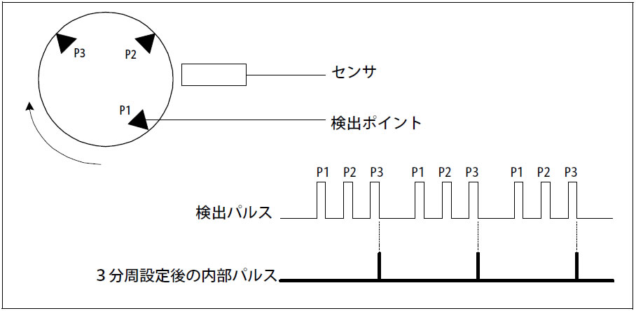 The division ratio can be set regardless of the input frequency and display value settings.
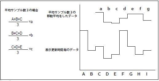
Moving Average
Updates output while averaging a specified number of sample data points.
This allows for smooth output while maintaining high-speed response to uneven flow rates.
The calculation takes one new measurement value and discards the oldest one at each output (display) update time for averaging.
Example: Output update time 0.1s, Average samples 3
A, B... are data (measurement values) for each update time.
While calculating the average for the past 0.3s, the output can respond every 0.1s update interval.
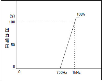
Spread
Allows for magnification of a specific frequency range. By defining upper and lower frequency limits,
frequency variations within that range can be output through a specified range (e.g., 0-10V, 4-20mA).
Example:
If Upper Limit is 1kHz and Lower Limit is 750Hz, it appears as shown below. However, since resolution decreases,
extreme magnification may lead to a loss of accuracy.
Dual Range
In addition to the full scale set in basic specifications, another full scale can be set to switch ranges.
This allows for alternating observation of two objects with different speeds, or viewing the vicinity of maximum and minimum speeds at different full scales.
Example: By setting two full scales (FS) at 1kHz and 10Hz, a 10Hz input will output 0.1V at 1kHz FS and 10V at 10Hz FS.
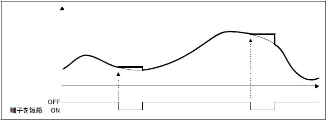
Current Value Hold
Short-circuiting (ON) the hold terminal maintains the current measurement output until it is turned OFF (H level).
Internal measurement calculations continue to run.
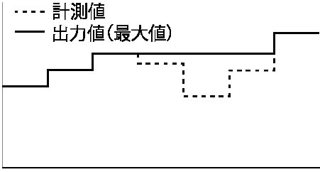
Max Value Hold
Updates and outputs only the maximum data value while the hold terminal is short-circuited (ON).
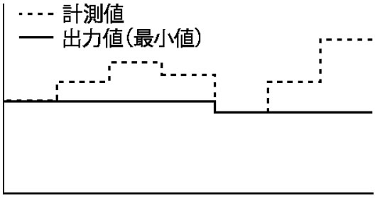
Min Value Hold
Updates and outputs only the minimum data value while the hold terminal is short-circuited (ON).
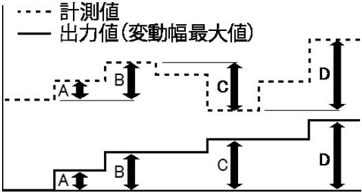
Max Variation Range Hold
Updates and outputs only the difference between the maximum and minimum values while the hold terminal is short-circuited (ON).
General-purpose Signals
Periodic signals including general pulses. If noise is superimposed on sine waves, etc.,
it may cause trigger timing shifts and measurement errors. Square wave input is recommended for accurate measurement.
Sine Wave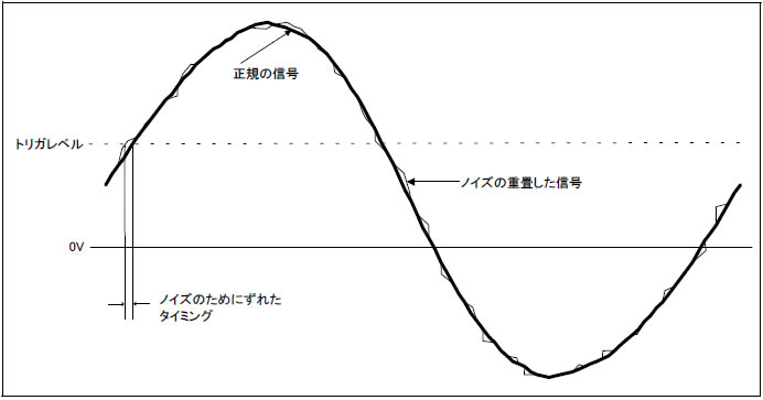 |
Square Wave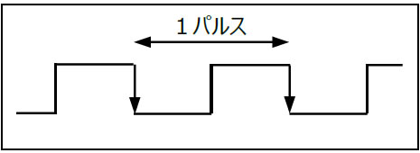 |
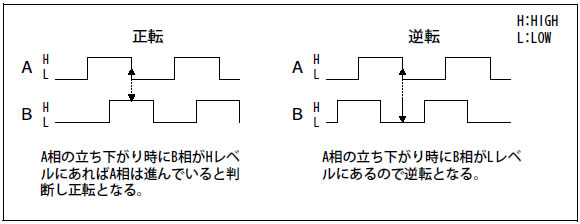
90° Phase Difference Signals (A/B Phase)
For bidirectional rotation measurement, two-phase pulses with a 90° phase difference are input.
Since there is a 90° phase difference, Phase A and Phase B do not change simultaneously. Direction can be determined by observing the rising edge of Phase A relative to Phase B.
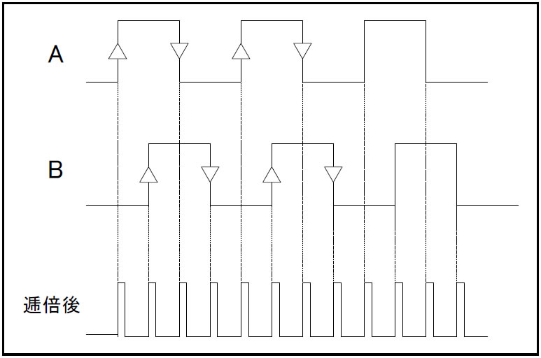
2-Phase 4-Multiplication (QUAD)
A 4x pulse multiplication function that utilizes the rising/falling edges of each phase pulse to internally quadruple the frequency.
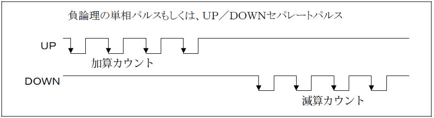
UP/DOWN Signals
For bidirectional counting, UP/DOWN separate pulses can be input in addition to 90° phase difference signals.
The pulse input sections for A: UP and B: DOWN are independent, measuring at the falling edge regardless of each other's logic.
[Note] Positive logic UP/DOWN signals cannot be input.
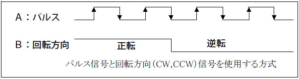
Directional Signals
Uses an independent pulse signal and a rotation direction signal.
> To "Trigger Level and Hysteresis" page
> To "Types of Pulse Signals" page
F/V Converter [Frequency-to-Voltage Converter] NEW
A device that takes speed information from moving objects (converted to pulses by proximity switches, optical sensors, encoders, gear sensors, etc.) and converts/outputs it as an analog voltage (or current) proportional to the speed is called an F/V Converter.
[Example of F/V Converter Application]
Gear sensors, etc. |
→→ |
 F/V Converter |
→→ |
 PC |
 Logger |
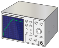 Oscilloscope, etc. |
Speed monitoring can be performed by connecting indicator instruments, and rotation variations can be observed by connecting to a recorder.
Connection to other control equipment for follow-up control is also possible.
> View F/V Converter Application Examples
Frequency Meters and Period Meters NEW
In general F/V converters, the voltage output varies in proportion to frequency.
Types where voltage increases in proportion to frequency are called frequency meters, including tachometers, flowmeters, and speedometers.
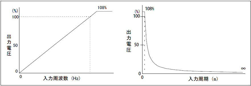 [Fig: Frequency Meter]
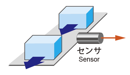
Types where voltage varies in proportion to the period are called period meters (or transit time meters),
used for measuring the time it takes for an object (including fluids) to pass over a conveyor, etc.
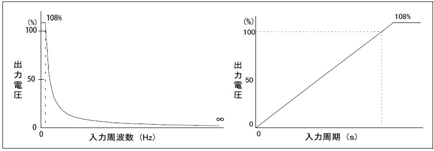 [Fig: Period Meter]
[Example Application Image]
|
→→ |
|
→→ |
PC |
Logger |
Oscilloscope, etc. |
> View Speedometer Application Examples
> View Flowmeter Application Examples
Full Scale
When converting frequency to voltage (current), you must decide what voltage (or current) to output at a specific frequency (Hz).
The maximum input frequency and its corresponding voltage (current) is called Full Scale.
Bias
The bias setting is a function for obtaining 1-5V or 4-20mA output for instrumentation purposes.
The setting range is 0-50%.
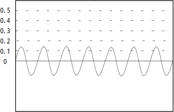
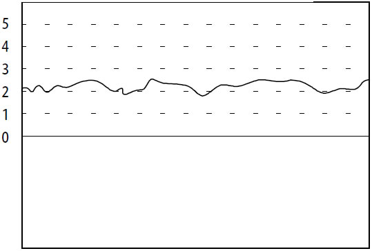
Input Coupling (AC/DC Coupling)
DC Coupling: Passes both DC and AC components.
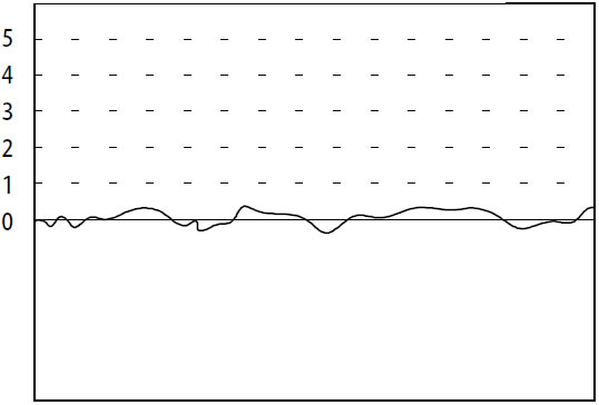
AC Coupling: Blocks the DC component.
AC is used when observing only the AC variation of an input signal that has an superimposed DC offset.
| DC Coupling | AC Coupling | |
 |
→ |  |
| ↓ Attempting to magnify the waveform by x10 causes the 2V region to go out of display range. |
↓ By cutting the DC component, only the AC variation can be magnified and observed. |
|
 |
 |
|
| DC Coupling | AC Coupling | |
 |
 |
|
| If the signal is unstable and triggers are hard to set, AC coupling sets the trigger level to 0V, stabilizing the waveform. |
Calibrate
When connecting measuring instruments to recorders, etc., correct results cannot be obtained unless the 0% and 100% values match precisely, making calibration necessary.
Devices with built-in calibrators generate a reference signal to adjust output at offset or full scale, and can also adjust connected equipment.
Rotary Encoders
The number of pulses per rotation can be selected according to application to increase resolution. Two-phase output types allow for direction detection.
They can be used as peripheral speed sensors with pulleys, etc. The shaft must be directly rotated via a coupling.
Proximity Sensors
Non-contact sensors that function even in harsh environments like oil contamination, but must be placed close (approx. 10mm or less) to the target.
Many are applicable to frequencies of 1kHz or less.
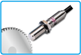
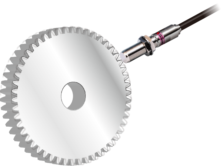
Gear Sensors NEW
The most common sensor used for digital tachometers, etc. Gate-type tachometers require 60 pulses per rotation; Module 1 gears (where pulse count equals diameter) are easy to use. High-sensitivity types are susceptible to noise; some models have built-in amplifiers.

 > View Gear Sensor List
> View Gear Sensor Application Examples
Photoelectric Sensors
Non-contact, easy to install, and low cost, but cannot be used in harsh environments like oil. Most support frequencies up to 1kHz.
Optical fiber types can separate the amplifier unit to remain unaffected by noise.
Various types exist, including retro-reflective types for proximity and laser types for small targets.
Flow Sensors NEW
Output pulses proportional to unit flow. Positive displacement types are highly accurate and cover a wide range from high to low flow rates.
In low flow regions, the pulse cycle may not be proportional to flow due to rotation unevenness in vanes, etc. (though proportional on average).
It may not be possible to obtain many pulses per rotation, and input signal wiring can become long.
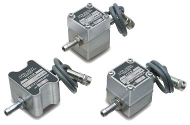 > View Flow Sensor List
[Operation Image of Positive Displacement Flow Sensor] *Example of COCORESEARCH XFS series
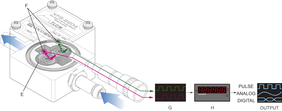
> View Principle of Operation (Example)
> Technical Information Page